Analyzing Similarities in Conversational Sequence in One Dyad

Introduction

This vignette demonstrates how to use the conversation similarity sequence functions provided in the package. These functions allow you to analyze various aspects of similarity in conversations over time, including topic, lexical, semantic, stylistic, and sentiment similarities.

Setup

First, let’s load the necessary libraries:

library(ggplot2)
library(tm)
library(conversim)

Sample Data

Let’s create a sample conversation dataset to work with:

set.seed(123)
conversation <- data.frame(
  speaker = rep(c("A", "B"), 10),
  processed_text = c(
    "Hello how are you today",
    "I'm doing well thanks for asking",
    "That's great to hear what are your plans",
    "I'm planning to go for a walk later",
    "Sounds nice the weather is beautiful",
    "Yes it's perfect for outdoor activities",
    "Do you often go for walks",
    "Yes I try to walk every day for exercise",
    "That's a great habit to have",
    "Thanks I find it helps me stay healthy",
    "Have you tried other forms of exercise",
    "I also enjoy swimming and yoga",
    "Those are excellent choices too",
    "What about you what exercise do you prefer",
    "I like running and playing tennis",
    "Tennis is fun do you play often",
    "I try to play at least once a week",
    "That's a good frequency to maintain",
    "Yes it keeps me active and social",
    "Social aspects of exercise are important too"
  )
)

Topic Similarity Sequence

Let’s start by analyzing the topic similarity sequence:

topic_sim <- topic_sim_seq(conversation, method = "lda", num_topics = 2, window_size = 3)

# Plot the topic similarity sequence
ggplot(data.frame(Segment = 1:3, Similarity = topic_sim$sequence), aes(x = Segment, y = Similarity)) +
  geom_line() +
  geom_point() +
  labs(title = "Topic Similarity Sequence", x = "Conversation Segment", y = "Similarity Score") +
  theme_minimal()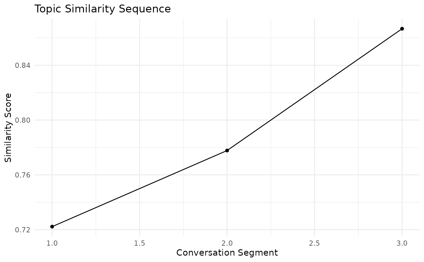

# Print the average topic similarity
cat("Average topic similarity:", round(topic_sim$average, 3))
#> Average topic similarity: 0.784

Lexical Similarity Sequence

Next, let’s look at the lexical similarity sequence:

lexical_sim <- lex_sim_seq(conversation, window_size = 3)

# Plot the lexical similarity sequence
ggplot(data.frame(Exchange = 1:length(lexical_sim$sequence), Similarity = lexical_sim$sequence), 
       aes(x = Exchange, y = Similarity)) +
  geom_line() +
  geom_point() +
  labs(title = "Lexical Similarity Sequence", x = "Conversation Exchange", y = "Similarity Score") +
  theme_minimal()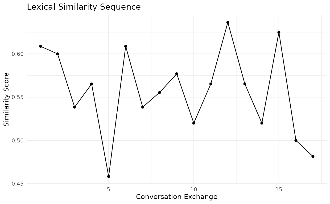

# Print the average lexical similarity
cat("Average lexical similarity:", round(lexical_sim$average, 3))
#> Average lexical similarity: 0.557

Semantic Similarity Sequence

Now, let’s analyze the semantic similarity sequence:

semantic_sim <- sem_sim_seq(conversation, method = "tfidf", window_size = 3)

# Plot the semantic similarity sequence
ggplot(data.frame(Exchange = 1:length(semantic_sim$sequence), Similarity = semantic_sim$sequence), 
       aes(x = Exchange, y = Similarity)) +
  geom_line() +
  geom_point() +
  labs(title = "Semantic Similarity Sequence", x = "Conversation Exchange", y = "Similarity Score") +
  theme_minimal()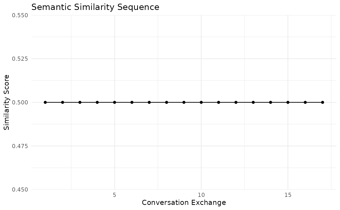

# Print the average semantic similarity
cat("Average semantic similarity:", round(semantic_sim$average, 3))
#> Average semantic similarity: 0.5

Stylistic Similarity Sequence

Let’s examine the stylistic similarity sequence:

stylistic_sim <- style_sim_seq(conversation, window_size = 3)

# Plot the stylistic similarity sequence
ggplot(data.frame(Exchange = 1:length(stylistic_sim$sequence), Similarity = stylistic_sim$sequence), 
       aes(x = Exchange, y = Similarity)) +
  geom_line() +
  geom_point() +
  labs(title = "Stylistic Similarity Sequence", x = "Conversation Exchange", y = "Similarity Score") +
  theme_minimal()

# Print the average stylistic similarity
cat("Average stylistic similarity:", round(stylistic_sim$average, 3))
#> Average stylistic similarity: 0.917

Sentiment Similarity Sequence

Finally, let’s analyze the sentiment similarity sequence:

sentiment_sim <- sent_sim_seq(conversation, window_size = 3)

# Plot the sentiment similarity sequence
ggplot(data.frame(Exchange = 1:length(sentiment_sim$sequence), Similarity = sentiment_sim$sequence), 
       aes(x = Exchange, y = Similarity)) +
  geom_line() +
  geom_point() +
  labs(title = "Sentiment Similarity Sequence", x = "Conversation Exchange", y = "Similarity Score") +
  theme_minimal()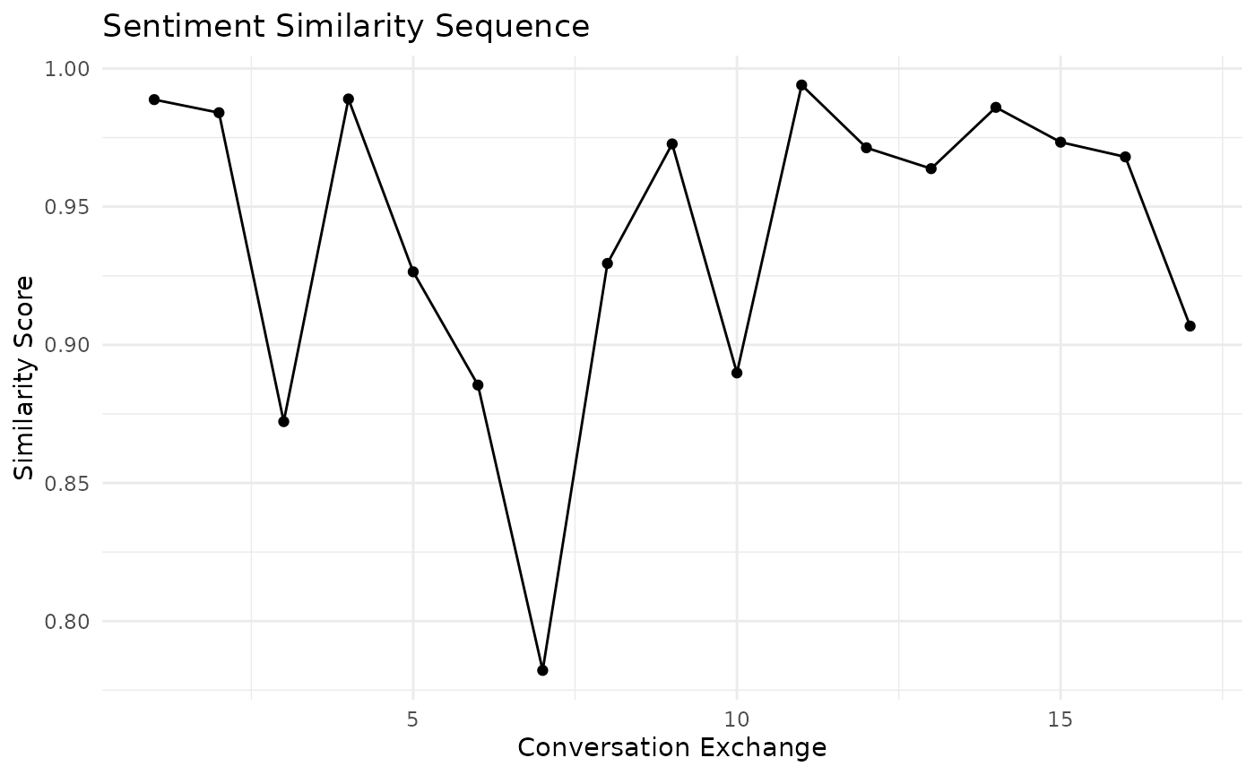

# Print the average sentiment similarity
cat("Average sentiment similarity:", round(sentiment_sim$average, 3))
#> Average sentiment similarity: 0.94

Conclusion

This vignette demonstrates how to use various functions to analyze different aspects of similarity in conversations. By examining topic, lexical, semantic, stylistic, and sentiment similarities, researchers can gain insights into the dynamics of conversations and how they evolve over time.

These tools can be particularly useful in fields such as linguistics, psychology, and communication studies, where understanding the nuances of conversation patterns is crucial.