Analyzing Similarities in Conversational Sequences across Multiple Dyads • conversim

Introduction

This vignette demonstrates how to use the functions provided in the conversation_multidyads.R file to analyze conversations across multiple dyads. These functions allow you to preprocess conversation data and calculate various similarity measures between conversation participants.

Setup

Load the library:

library(conversim)

Loading the Data

We’ll use the provided dataset “dyad_example_data.Rdata” located in the inst/extdata directory of the package:

data_path <- system.file("extdata", "dyad_example_data.Rdata", package = "conversim")
load(data_path)

# Display the first few rows and structure of the data
head(dyad_example_data)
#> # A tibble: 6 × 3
#>   dyad_id speaker_id text                                                       
#>     <dbl> <chr>      <chr>                                                      
#> 1       1 A          What did you think of the new movie that just came out?    
#> 2       1 B          I haven’t seen it yet. Which one are you referring to?     
#> 3       1 A          The latest superhero film. I heard it’s getting great revi…
#> 4       1 B          Oh, that one! I’ve been meaning to watch it. Did you enjoy…
#> 5       1 A          Yes, I thought it was fantastic. The special effects were …
#> 6       1 B          Really? What about the storyline? I heard it’s a bit predi…
str(dyad_example_data)
#> tibble [532 × 3] (S3: tbl_df/tbl/data.frame)
#>  $ dyad_id   : num [1:532] 1 1 1 1 1 1 1 1 1 1 ...
#>  $ speaker_id: chr [1:532] "A" "B" "A" "B" ...
#>  $ text      : chr [1:532] "What did you think of the new movie that just came out?" "I haven’t seen it yet. Which one are you referring to?" "The latest superhero film. I heard it’s getting great reviews." "Oh, that one! I’ve been meaning to watch it. Did you enjoy it?" ...

Preprocessing

Before analyzing the conversations, we need to preprocess the text data:

processed_convs <- preprocess_dyads(dyad_example_data)
head(dyad_example_data)
#> # A tibble: 6 × 3
#>   dyad_id speaker_id text                                                       
#>     <dbl> <chr>      <chr>                                                      
#> 1       1 A          What did you think of the new movie that just came out?    
#> 2       1 B          I haven’t seen it yet. Which one are you referring to?     
#> 3       1 A          The latest superhero film. I heard it’s getting great revi…
#> 4       1 B          Oh, that one! I’ve been meaning to watch it. Did you enjoy…
#> 5       1 A          Yes, I thought it was fantastic. The special effects were …
#> 6       1 B          Really? What about the storyline? I heard it’s a bit predi…

Calculating Similarities

Now, let’s calculate various similarity measures for our preprocessed conversations.

Topic Similarity

topic_sim <- topic_sim_dyads(processed_convs, method = "lda", num_topics = 5, window_size = 3)

Lexical Similarity

lexical_sim <- lexical_sim_dyads(processed_convs, window_size = 3)

Semantic Similarity

semantic_sim <- semantic_sim_dyads(processed_convs, method = "tfidf", window_size = 3)

Structural Similarity

structural_sim <- structural_sim_dyads(processed_convs)

Stylistic Similarity

stylistic_sim <- stylistic_sim_dyads(processed_convs, window_size = 3)

Sentiment Similarity

sentiment_sim <- sentiment_sim_dyads(processed_convs, window_size = 3)

Participant Similarity

participant_sim <- participant_sim_dyads(processed_convs)

Timing Similarity

timing_sim <- timing_sim_dyads(processed_convs)
#> Warning in timing_sim_dyads(processed_convs): Only one observation per dyad.
#> Using simple mean for overall average instead of multilevel modeling.

Visualization

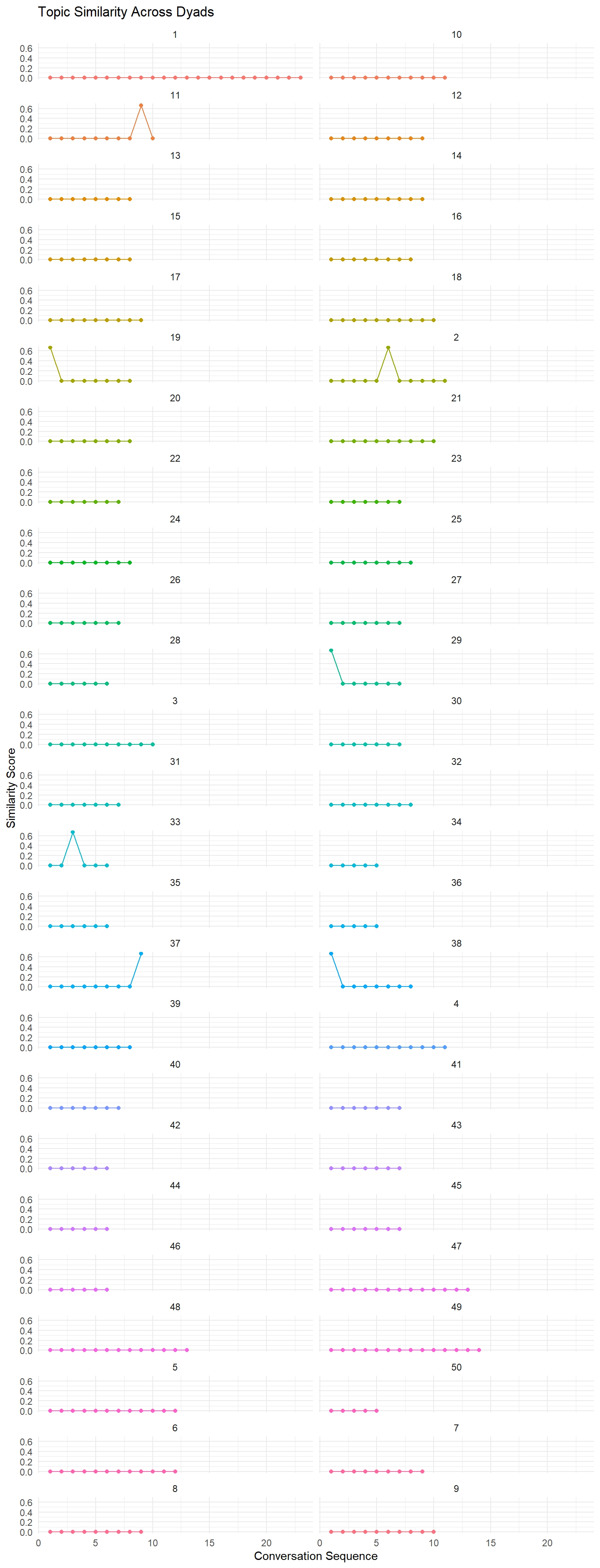
Let’s visualize the results of our similarity analyses using ggplot2. Here’s an example of how to plot the topic similarity for each dyad:

topic_sim_df <- data.frame(
  dyad = rep(names(topic_sim$similarities_by_dyad), 
             sapply(topic_sim$similarities_by_dyad, length)),
  similarity = unlist(topic_sim$similarities_by_dyad),
  index = unlist(lapply(topic_sim$similarities_by_dyad, seq_along))
)

ggplot(topic_sim_df, aes(x = index, y = similarity, color = dyad)) +
  geom_line() +
  geom_point() +
  facet_wrap(~dyad, ncol = 2) +
  labs(title = "Topic Similarity Across Dyads",
       x = "Conversation Sequence",
       y = "Similarity Score") +
  theme_minimal() +
  theme(legend.position = "none")

Comparing Different Similarity Measures

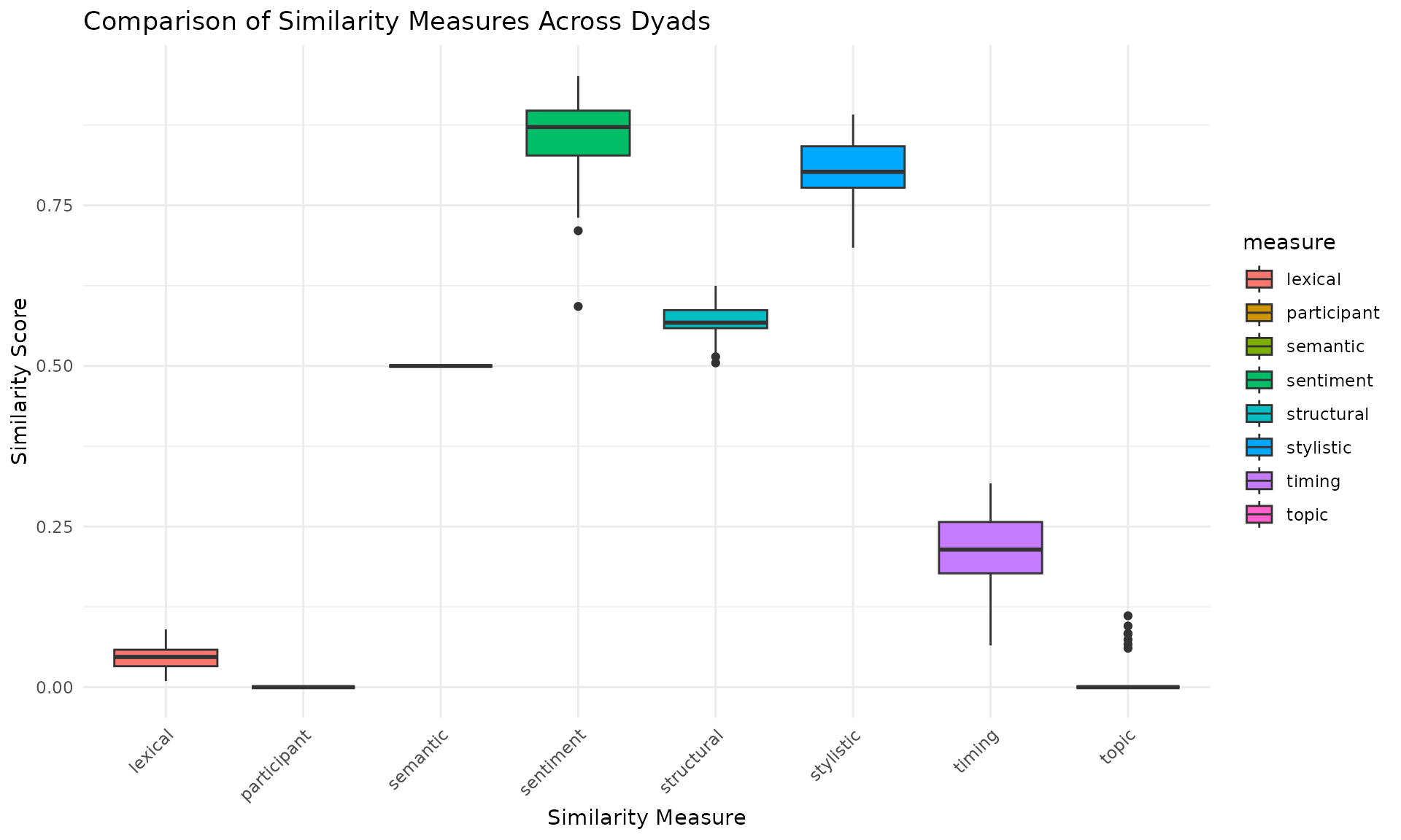
We can also compare different similarity measures across dyads:

comparison_df <- data.frame(
  dyad = names(topic_sim$similarities_by_dyad),
  topic = sapply(topic_sim$similarities_by_dyad, mean),
  lexical = sapply(lexical_sim$similarities_by_dyad, mean),
  semantic = sapply(semantic_sim$similarities_by_dyad, mean),
  structural = unlist(structural_sim$similarities_by_dyad),
  stylistic = sapply(stylistic_sim$similarities_by_dyad, mean),
  sentiment = sapply(sentiment_sim$similarities_by_dyad, mean),
  participant = unlist(participant_sim$similarities_by_dyad),
  timing = unlist(timing_sim$similarities_by_dyad)
)

comparison_long <- reshape(comparison_df, 
                           varying = list(names(comparison_df)[names(comparison_df) != "dyad"]),
                           v.names = "similarity",
                           timevar = "measure",
                           times = names(comparison_df)[names(comparison_df) != "dyad"],
                           new.row.names = 1:10000, # Adjust this if needed
                           direction = "long")

ggplot(comparison_long, aes(x = measure, y = similarity, fill = measure)) +
  geom_boxplot() +
  labs(title = "Comparison of Similarity Measures Across Dyads",
       x = "Similarity Measure",
       y = "Similarity Score") +
  theme_minimal() +
  theme(axis.text.x = element_text(angle = 45, hjust = 1))

Conclusion

This vignette demonstrates how to use the functions in conversation_multidyads.R to analyze conversations across multiple dyads using real-world data. These tools allow researchers to examine various aspects of conversation dynamics, including topic coherence, lexical alignment, semantic similarity, and more.

The visualizations provide insights into how different similarity measures vary across dyads and how they compare to each other. This can help in identifying patterns or trends in conversational dynamics.

Remember that the effectiveness of these analyses may depend on the size and nature of your dataset. Always consider the context of your conversations and the limitations of each similarity measure when interpreting the results.

For further analysis, you might consider:

Investigating dyads with particularly high or low similarity scores.
Examining how similarity measures change over the course of conversations.
Correlating similarity measures with other variables of interest (e.g., conversation outcomes, participant characteristics).